This is the first set of a series of graph search algorithms that I will examine. I describe breadth first search and depth first search and implement them to find paths between cities and solutions to mazes.
While relatively simple, these algorithms form the foundations of many more sophisticated techniques for optimization. I begin here by describing and programming two uninformed search methods: breadth first search and depth first search. Both graph searches are complete, but not necessarily optimal. The algorithms are demonstrated by finding solutions to a graph of connected cities as well as a maze.
Breadth First Search
In Breadth-first search (BFS), the root node is expanded first, then the successors of the root, then the successors of the successors of the root, and so on, until the goal is reached. BFS finds the shallowest path to each node from the frontier, so it is best used on graphs where the goal is close to the start. For example, it could be useful when finding close connections on social media. BFS is optimal when all path lengths are equal. A queue (FIFO) is used to implement BFS to expand the shallowest nodes first. The space complexity of BFS is exponential, O(b^d)., where b is the branching factor and d is the depth of the solution.
def breadth_first(start, goal, state_graph, return_cost=False):
    frontier = [start]
    visited = [start]
    parent = {start:None}

    if start == goal:
        solution = path(parent, goal)
        if(return_cost == False):
            return solution
        else:
            try:
                solution_cost = pathcost(solution, state_graph)
            except:
                solution_cost = 0
            return solution, solution_cost

    while frontier:
        currNode = frontier.pop(0)

        for child in state_graph[currNode]:
            if child not in visited:
                visited.append(child)
                parent[child] = currNode
                frontier.append(child)
            if child == goal:
                bfs_path = get_path(start, goal, parent)
                solution = path(bfs_path, goal)
                if(return_cost==False):
                    return solution
                else:
                    try:
                        solution_cost = pathcost(solution, state_graph)
                    except:
                        step_cost = 1
                        solution_cost = step_cost*(len(solution))
                    return solution, solution_cost
    return 0
Depth First Search
Depth-first search (DFS) traverses down a branch to a node furthest from the root before backtracking. For this reason, it is better when used on searches for which the goal is far from the start. It is very similar to a BFS, but is implemented using a stack (LIFO), so it the deepest nodes will be expanded first. DFS can also be implemented recursively. Since DFS only needs to store a single path from the root to a leaf node, the standard DFS actually has a much better space complexity than BFS, O(bm), where m is the maximum depth of any node. Unfortunately, the algorithm fails in the case of an infinite-depth space; as a result, it is non-optimal.
def depth_first(start, goal, state_graph, return_cost=False):
    parent = {start:None}
    frontier = [start]
    visited = []

    if start == goal:
        solution = path(parent, goal)
        if(return_cost == False):
            return solution
        else:
            try:
                solution_cost = pathcost(solution, state_graph)
            except:
                solution_cost = 0
            return solution, solution_cost

    while frontier:
        currNode = frontier.pop()
        visited.append(currNode)
        for child in state_graph[currNode]:
            if child not in visited:
                parent[child] = currNode
                frontier.append(child)
                if child == goal:
                    visited.append(goal)
                    dfs_path = get_path(start, goal, parent)
                    solution = path(dfs_path, goal)
                    if(return_cost==False):
                        return solution
                    else:
                        try:
                            solution_cost = pathcost(solution, state_graph)
                        except:
                            step_cost = 1
                            solution_cost = step_cost*(len(solution))
                        return solution, solution_cost
    return 0
Usage
Weighted Graph
BFS and DFS are demonstrated on a graph of US cities. Note that while the paths between nodes have costs, the path costs are not used by either algorithm when selecting nodes to visit, only for calculating the final found path cost. The graph is represented programmatically as a dictionary.
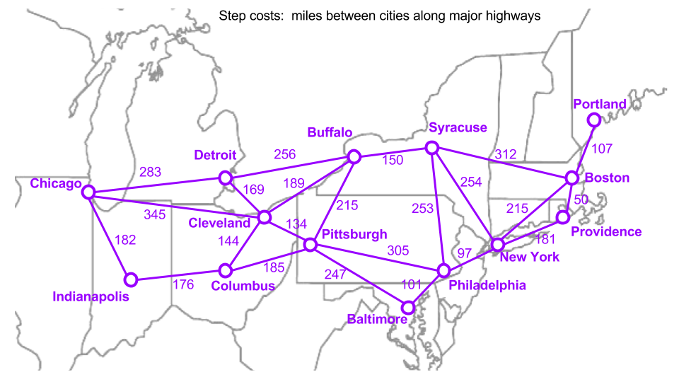
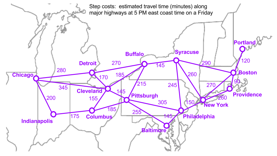
Using the algorithms to find a path from Chicago to New York using two different weights for the graph, distances and times:
Distances:
Breadth First Path = ['chi', 'det', 'buf', 'syr', 'new'] , Distance (miles) = 943
Depth First Path = ['chi', 'ind', 'col', 'pit', 'bal', 'phi', 'new'] , Distance (miles) = 988
Times:
Breadth First Path = ['chi', 'det', 'buf', 'syr', 'new'] , Time (mins) = 955
Depth First Path = ['chi', 'ind', 'col', 'pit', 'bal', 'phi', 'new'] , Time (mins) = 1110
Solving a maze
I used BFS and DFS to find solutions to a maze. The maze is represented using a binary numpy array where 1s represent walls and 0s represent open space.
First, I converted the maze to a dictionary that listed possible actions from each valid position in the maze and then used BFS and DFS to solve. Then I wrote a function to plot the maze and the found path.
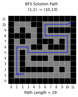
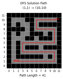
Below, BFS and DFS are demonstrated on a maze where the goal is to get from the start at (1,1) to the finish at (10,10). Note that since the path costs are all equal, BFS finds the optimal solution in this case.
breadth_first((1,1), (10,10), maze_graph, True)
depth_first((1,1), (10,10), maze_graph, True)

BFS Solution = [(1, 1), (1, 2), (1, 3), (1, 4), (1, 5), (1, 6), (2, 6), (3, 6), (3, 5), (4, 5), (5, 5), (6, 5), (7, 5), (8, 5), (9, 5), (10, 5), (10, 6), (10, 7), (10, 8), (9, 8), (8, 8), (7, 8), (6, 8), (6, 9), (6, 10), (7, 10), (8, 10), (9, 10), (10, 10)] , Path Length = 29

DFS Solution = [(1, 1), (2, 1), (3, 1), (4, 1), (5, 1), (6, 1), (7, 1), (8, 1), (9, 1), (10, 1), (10, 2), (10, 3), (9, 3), (8, 3), (7, 3), (6, 3), (5, 3), (4, 3), (3, 3), (3, 4), (3, 5), (4, 5), (5, 5), (6, 5), (7, 5), (8, 5), (9, 5), (10, 5), (10, 6), (10, 7), (10, 8), (9, 8), (8, 8), (7, 8), (6, 8), (6, 9), (6, 10), (7, 10), (8, 10), (9, 10), (10, 10)] , Path Length = 41
These helper functions below are used in the algorithms above.
def path(previous, s):
    '''
    `previous` is a dictionary chaining together the predecessor state that led to each state
    `s` will be None for the initial state
    otherwise, start from the last state `s` and recursively trace `previous` back to the initial state,
    constructing a list of states visited as we go
    '''
    if s is None:
        return []
    else:
        return path(previous, previous[s])+[s]

def pathcost(path, step_costs):
    '''
    add up the step costs along a path, which is assumed to be a list output from the `path` function above
    '''
    cost = 0
    for s in range(len(path)-1):
        cost += step_costs[path[s]][path[s+1]]
    return cost

    #path from destination to source
def get_path(start, goal, parent):
    invpath = {goal:parent[goal]}
    found_path=dict()
    while goal != start:
        goal = parent[goal]
        invpath[goal] = parent[goal]
    for k in reversed(list(invpath.keys())):
        found_path[k] = invpath[k]
    return found_path
These algorithms were originally programmed in an Artificial Intelligence class in Fall 2020 and improved/modified for this post.
