
This is the second set of a series of graph search algorithms I will examine. Here, two informed graph search methods– Uniform Cost Search and A star– will be described and programmed. The algorithms are demonstrated on two different weighted undirected graphs and to find the optimal path on a maze-like map.
These algorithms improve upon BFS and DFS to create more efficient and powerful search methods. Breadth-first search is only optimal when all path costs are equal. Uniform Cost Search expands on Breadth-first search by solving the non-optimality when all path costs are not equal by always taking the shortest available path. Furthermore, BFS selects the goal node when it first appears (as a child of a parent node), which could result in a sub-optimal path. UCS will only select the goal node when it is selected for expansion in the priority queue. UCS is optimal!
I start by creating a class called Frontier_PQ to represent the frontier (a priority queue) for both Uniform Cost Search and A* Search. The priority queue is sorted in order of lowest cost to greatest cost and is implemented as a heap. There is some redundancy in the information stored in states and q. This redundancy could be eliminated to reduce storage requirements, however, it would increase the time complexity as the priority queue would need to be checked for states.
# Takes instantiation arguments state, cost
# start is the initial state(e.g. start='chi'), cost is the initial path cost
class Frontier_PQ:
# instantiation arguments
    def __init__(self, start, cost):
        self.start = str(start)
        self.cost = str(cost)
        self.states = {}
        self.q = [(cost,start)]
        heapq.heapify(self.q)

# add (cost, state) tuple to the frontier
    def add(self, state, cost):
        heapq.heappush(self.q,(cost, state))
        return

# return the lowest-cost tuple and pop it off the frontier
    def pop(self):
        lowest_cost_node = heapq.heappop(self.q)
        state = lowest_cost_node[1]
        cost = lowest_cost_node[0]
        return lowest_cost_node

# if a lower-cost path to a state that is already on the frontier, replace it and re-sort the priority queue
    def replace(self, state, cost, index):
        self.q[index]=(cost, state)
        self.q.sort()
        return
Uniform Cost Search
My code for UCS is given below.
start: initial state
goal: goal state
state_graph: graph representing the connectivity and step costs of the state space
return_cost: logical input of whether or not to return the solution path cost
return_nexp: logical input of whether or not to return the number of nodes expanded by the algorithm
def uniform_cost(start, goal, state_graph, return_cost=False, return_nexp=False):
# initialize
    parent = {start:None}
    frontier = Frontier_PQ(start, 0)
    visited = [start]
    found_path = []
    nodes_expanded = 0
# select node to be expanded, based on cost
    while frontier.q:
        if not frontier.q:
            print("Failure!")
            return
        currNode = frontier.pop() #pop lowest cost node
        currCity = currNode[1]
        cost = currNode[0]
        found_path = found_path + [currCity]
        if currNode[1] not in visited:
            visited.append(currNode[1])
# goal state is selected to be expanded, terminate
        if currCity == goal:
            ucs_path = get_path(start, goal, parent)
            solution = path(ucs_path, goal)
            solution_cost = cost
            solution_cost2 = pathcost(solution, state_graph)
            if solution_cost != solution_cost2:
                print("Failure")
                return
            nodes_expanded = len(visited)-1
            if(return_cost==False and return_nexp==False):
                return solution
            elif(return_cost==True and return_nexp==False):
                return [solution, solution_cost]
            elif(return_cost==False and return_nexp==True):
                return [solution,None ,nodes_expanded]
            elif(return_cost==True and return_nexp==True):
                return [solution, solution_cost, nodes_expanded]
# check children, add them and costs to the frontier
        for child in state_graph[currNode[1]]:
            child_cost = state_graph[currNode[1]][child]
            ttl_cost = cost+child_cost
            childNode = (cost, child)
            if (child not in visited) and (child not in frontier.states): #frontier.states
                frontier.add(child, ttl_cost)
                frontier.states[child] = ttl_cost
                parent[child]=currCity
            elif (child in frontier.states) and (ttl_cost < frontier.states[child]):
                index = frontier.q.index((frontier.states[child], child))
                frontier.replace(child, ttl_cost, index)
                frontier.states[child] = ttl_cost
                parent[child]=currCity
    return 0
The A* Search algorithm improves upon UCS by using outside information, called a heuristic to guide the search and improve efficiency. A* search is an informed search algorithm, while the previous searches have been uninformed techniques. The heuristic is said to be admissible if it never overestimates the cost of reaching the goal. It must be admissible for an algorithm to be optimal.
A* Search
def astar_search(start, goal, state_graph, heuristic, return_cost=False, return_nexp=False):
# initialize
    parent = {start:None}
    frontier = Frontier_PQ(start, 0)
    visited = [start]
    found_path = []
    nodes_expanded = 0
# select node to be expanded, based on true costs and heuristic
    while frontier.q:
        if not frontier.q:
            print("Failure!")
            return
        currNode = frontier.pop() #pop lowest cost node
        currCity = currNode[1]
        cost = currNode[0]+heuristic(currNode[1])
        found_path = found_path + [currCity]
        nodes_expanded +=1
        if currNode[1] not in visited:
            visited.append(currNode[1])
# goal state is selected to be expanded, terminate
        if currCity == goal:
            astar_search = get_path(start, goal, parent)
            solution = path(astar_search, goal)
            solution_cost = pathcost(solution, state_graph)
            nodes_expanded = len(visited)-1
            if(return_cost==False and return_nexp==False):
                return solution
            elif(return_cost==True and return_nexp==False):
                return [solution, solution_cost]
            elif(return_cost==False and return_nexp==True):
                return [solution,None ,nodes_expanded]
            elif(return_cost==True and return_nexp==True):
                return [solution, solution_cost, nodes_expanded]
# check children, add them and heuristic+costs to the frontier
        for child in state_graph[currNode[1]]:
            child_cost = state_graph[currNode[1]][child]
            ttl_cost = currCost+child_cost+heuristic(child)
            childNode = (cost, child)
            if (child not in visited) and (child not in frontier.states):
                frontier.add(child, ttl_cost)
                frontier.states[child] = ttl_cost
                parent[child]=currCity
            elif (child in frontier.states) and (ttl_cost < frontier.states[child]):
                frontier.replace(child, ttl_cost)
                frontier.states[child] = ttl_cost
                parent[child]=currCity
    return 0
Additional helper functions used are included in the previous Graph Search Algorithms post. They are pretty straightforward.
Usage
Run all of the algorithms above on a weighted graph of US cities. map_distances is implemented as a dictionary of connected nodes.
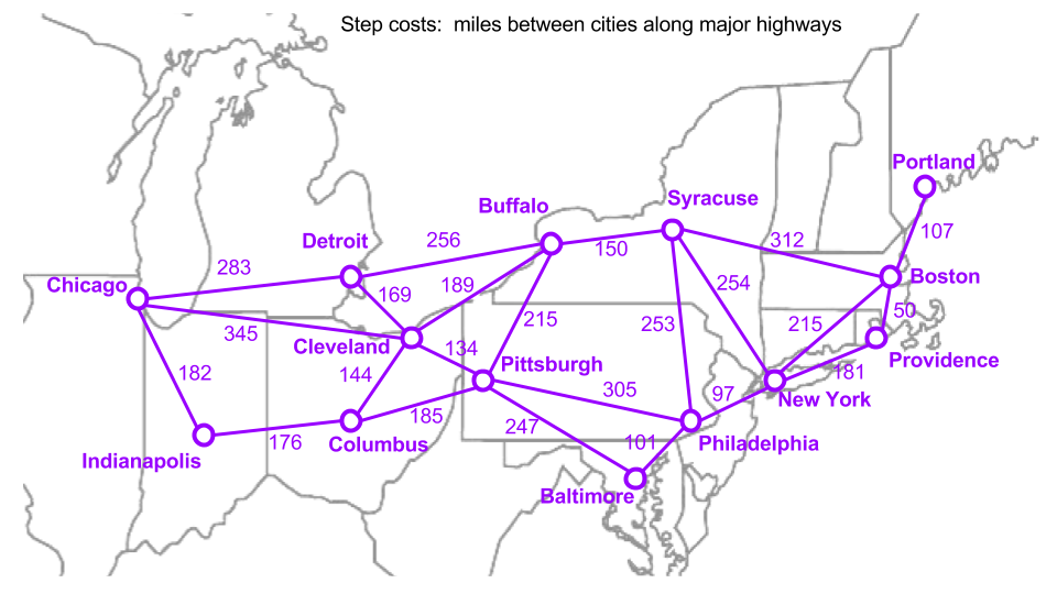
Weighted Graph
Find the optimal path from Chicago to Providence using the straight-line distance to Providence as a heuristic.
astar_path = astar_search('chi', 'pro', map_distances, heuristic_sld_providence, True, True)
ucs_path = uniform_cost('chi', 'pro', map_distances, True, True)

print("A* Search Path =", astar_path[0], ", Distance (miles) =", astar_path[1], ", Nodes Expanded =", astar_path[2], "\n")
print("Uniform Cost Search Path =", ucs_path[0], ", Distance (miles) =", ucs_path[1], ", Nodes Expanded =", ucs_path[2])
A* Search Path = ['chi', 'cle', 'buf', 'syr', 'bos', 'pro'] , Distance (miles) = 1046 , Nodes Expanded = 11

Uniform Cost Search Path = ['chi', 'cle', 'buf', 'syr', 'bos', 'pro'] , Distance (miles) = 1046 , Nodes Expanded = 12
Note that the optimal path found by both algorithms is the same, as it should be, but the A* Search was more efficient, because it expanded fewer nodes.
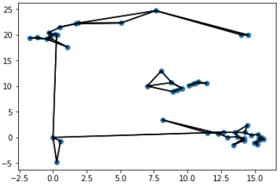
Another Weighted Graph
I used A* to get from the point $(0,0)$ to $(14,20)$ on the graph below using straight-line distance to the goal as the heuristic. I wrote a function to create the dictionary that represented the graph and then found the optimal path using A*.
astar_solution = astar_search((0,0), (14,20), distances, heuristic_fcn, return_cost=True)
print("A* Search Path =", astar_solution[0], " \nDistance (miles) =", astar_solution[1], "\n")
A* Search Path = [(0, 0), (0.2642182015052627, 20.033324445709404), (0.12547249447310752, 20.094573462136015), (-0.3326842354101051, 20.389978395358476), (0.5143024492904715, 21.50027514839235), (1.879542571484297, 22.29458591203462), (7.635895005315472, 24.701023330981783), (14, 20)]
Distance = 37.85905887568911
A Graph with a Larger State Space
Here I use A* search with the maximum of the number of rows, the number of columns, and the Euclidean distance from the goal, as the heuristic to get to from an initial state at $(1,15)$ to the goal state at $(25,9)$. In this scenario, diagonal movements are also allowed. Instead of building up the entire state space graph in memory as done previously, ONLY a partial state graph is given for each node expansion, with only neighboring states included.
The found solution is plotted below in black using a function I wrote. It has a path cost of 26.4853.
astar_path = astar_search((1,15), (25,9), adjacent_states, heuristic_max, return_cost=True, return_nexp=False)
print("optimal path =", astar_path[0], "\ncost =", astar_path[1])
optimal path = [(1, 15), (2, 15), (3, 15), (4, 15), (5, 15), (6, 15), (7, 15), (8, 15), (9, 15), (10, 15), (11, 15), (12, 15), (13, 15), (14, 15), (15, 14), (16, 13), (17, 13), (18, 12), (19, 12), (20, 11), (21, 10), (22, 10), (23, 10), (24, 9), (25, 9)]
cost = 26.485281374238575
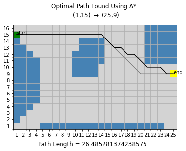
Notice there are many possible unique optimal paths (with the same cost) from the start to the goal other than the one found by my A* algorithm. Another optimal path from $(1,15)\rightarrow(14,15)\rightarrow(20,9)\rightarrow(25,9)$ is plotted above in gray.
These algorithms were originally programmed in an Artificial Intelligence class in Fall 2020 and improved/modified for this post.