In this third series on graph search algorithms, I use simulated annealing to find solutions to the traveling salesman problem.

Simulated Annealing (SA)

The goal of the traveling salesman problem is pretty simple: Find the shortest possible path between all n nodes in a graph and end at the start point. For this problem, the state space is discrete and there are (n-1)! possible solution paths (the problem is NP-Hard). The exponential rate of growth of the size of the state space makes it very difficult and in many cases not possible to find every solution path and then pick the optimal one. Simulated annealing is an optimization technique that avoids generating and storing every possible path combination to find a solution and works well with problems with discrete solution spaces. Because it does not solve the state space, SA is not necessarily optimal and often gives solutions that are close to the global minimum for practical purposes. The algorithm is named after the technique in metallurgy, which uses heating and cooling to reduce defects in metals. A metal is heated and cooled iteratively and then checked to see if its defects were reduced. Each heat/cool cycle is analogous to checking a new solution and seeing if it is better or worse (and sometimes taking a worse solution) in the SA algorithm.

SA begins with some initial solution and for each iteration, the algorithm finds a neighboring solution and always takes the solution if it is better than the current solution. If the neighboring solution is worse than the current solution, it is accepted with probability p, where p decays in time. This method creates a balance between exploitation (finding better solutions near our current state) and exploration (searching further for possible better solutions). The algorithm is able to explore and get out of local minimums effectively by taking worse solutions that may represent a better long term gain with a higher probability, then towards the end once it is (hopefully) close to the global minimum the probability it takes worse solutions is very low. The algorithm will also be given a temperature function T which determines how large of a change is allowed. Large changes are allowed at the beginning, but only smaller changes are allowed towards the end. Then, probability and temperature are related so that the algorithm takes solutions that are slightly worse with a greater probability than solutions that are MUCH worse.

Temperature and Probability Functions

Temperature Function

The temperature function chosen was $T(t)=\frac{C}{(t+1)^p}$, where $t$ is time and $C$ and $p$ are tunable constants. As $t\rightarrow n_{iterations}$, the temperature will decay to 0. The temperature tells us how far from the current state we are allowed to propose new candidates. Thus, a decaying temperature allows for very large changes initially and only small, local changes towards the end. A high temperature means to explore states all over the function and check them. Since the value $C \approx$ the largest value of the temperature, the value $C$ represents the largest change we are allowed to make at the beginning. I found $C\approx\sqrt{57}\approx7$ (57 nodes in the graph) seemed to work well for 100,000 iterations through trial and error. Then, I adjusted $p$ so that $p_{accept}$ looked reasonable (explanation below). The choice for $p$ was dependent on the max number of iterations.

Probability of Acceptance Function

The probability of acceptance function chosen was $p_{accept}=e^{\frac{\Delta E}{T(t)}}$, where $\Delta E = \text{objective_function}(current state) - \text{objective_function}(proposed state)$ and $T(t)$ is the temperature function. Note that when the cost of the current state is better than the cost of the proposed state $\Delta E >0$ and when the cost of the proposed state is better than the cost of the current state $\Delta E < 0$. We set $p_{accept}=1$ when the current state is better and $0<p_{accept} \le 1$ and decays when the proposed state is better than or equal to the current state. Additionally, note that (if $\Delta E <0$) the worse the proposed state is compared to the current state, the faster $p_{accept}$ decays; this means that the probability of acceptance of much worse proposed solutions will decrease much more quickly than the probability of acceptance of slightly worse proposed solutions (though the probabilities of both still decrease).

The behavior of this function, in theory, depends on the sign of $\Delta E$. However since I really only care about the value of $p_{accept}$ when the proposed state is worse than the current state (otherwise it is just 1), I only consider the case when $\Delta E < 0 \Rightarrow p_{accept}=e^{\frac{\Delta E}{T(t)}}$.

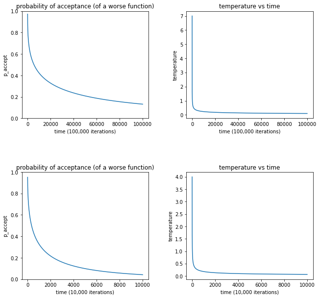
In the graphs below, I chose to test $p_{accept}$ with a $\Delta E = 0.2$. Through trial and error, I learned that a smooth decay of $p_{accept}$ (i.e. didn’t decay too quickly) worked best. Additionally, I found that if the difference between the proposed state and the current state is a path cost of 0.2, a probability of acceptance somewhere between 10% and 20% worked best.

This resulted in a choice of $C=7$ and $P=0.37$ for $n_{iterations} = 100,000$ and a choice of $C=4$ and $P=0.45$ for $n_{iterations} = 10,000$. The temperature functions and probability of acceptance functions for the two choices of stopping iterations are plotted below.

Annealing Implementation

First, I define an annealing class with attributes initial_state, current_state, best_state, objective_function, and schedule_function.

class state:
    #keep track of states- the current path and its cost/value
    def __init__(self, path, value):
        self.path = path
        self.value = value
                       
class problem_annealing:
    # Define the problem
    def __init__(self, initial, best, objective_function, schedule_function):
        self.initial_state = initial # a path that visits all the nodes. This will just be the list of nodes how they are.
        self.current_state = initial # the current path we are checking
        self.best_state = best # the best state we have found so far
        self.objective_function = objective_function # minimize the total path cost, this will be the path_cost() function.
        self.schedule_function = schedule_function # schedule function and probability of acceptance function, the information we need to choose our action
        
#for annealing: moves are somehow random: we will use temperature schedule to change candidates for all_moves
    def random_move(self):
        numNodes = len(self.current_state.path)
        newPath = self.current_state.path.copy()
        
        strReverseStart= np.random.randint(0, numNodes-1) #should be a random number from 0 to 56, don't include last node
        strReverseEnd= np.random.randint(2, numNodes-1)
        
        while strReverseEnd <= strReverseStart:
            strReverseStart= np.random.randint(0, numNodes-1)
            strReverseEnd= np.random.randint(2, numNodes-1)
            
        reverse_string(newPath, strReverseStart, strReverseEnd)

        newPath[57] = newPath[0]
        nextMove = newPath
        return nextMove, self.objective_function(nextMove)

Define some helper functions:

def make_graph(nodes):
    '''This function just makes the additional graph connections for the traveling salesman problem.'''
    graphDict={} # big dictionary
    numNodes = len(nodes)
    for n in nodes:
        graphDict[(n[0],n[1])]={}
    distancesList = np.zeros((numNodes,3))
    distancesList = distancesList.astype('object')
    
    for n in nodes: # each node should have a smaller dictionary, connecting it to its two closest nodes
        i=0
        temp = {}
        for m in nodes:
            dist = distance_formula(n, m) #Find distance between all pts connected to point n
            distancesList[i][0]= n
            distancesList[i][1]= m
            distancesList[i][2]= dist
            i+=1

        df= pd.DataFrame(data=distancesList, columns=['currPoint','nextPoint', 'distance'])
        df = df.astype({'distance': float,} ) #Convert object type of 'distance' column to float
        df = df[df.distance != 0.0] # Removes rows with a distance of 0 from the dataframe (this is the node itself)
        
        # This runs for EACH n.
        for i in range(numNodes-1):
            cx = df.values[i][1][0] #x-val of neighboring point
            cy = df.values[i][1][1] #y-val of neighboring point
            temp[(cx, cy)] = df.values[i][2] #
        graphDict[(n[0],n[1])] = temp
            
    return graphDict

def create_initial_path(nodes):
    # create a list of nodes in the form of the desired solution
    # i.e. a list of every node, beginning at one (arbitrarily chosen)node and ending at that same node
    numNodes = len(nodes)
    path = np.zeros(numNodes+1)
    path = path.astype('object')
    for i in range(numNodes):
        path[i] = (nodes[i][0], nodes[i][1])
    path[numNodes] = (nodes[0][0],nodes[0][1])
    return path

def reverse_string(array, strStart, strEnd):
    temp = array[strStart:strEnd]
    array[strStart:strEnd] = temp[::-1]
    return

Define a schedule function:

def schedule(time, C=C_input, p=p_input):
    '''some sort of mapping from time to temperature, to represent "cooling off" - 
    that is, accepting wacky solutions with lower and lower probability as time increases'''
    T = C/(time+1)**p #temperature
    return T

Finally, write simulated annealing.

def simulated_annealing(problem, n_iter):
    current_state = problem.initial_state
    best_state = problem.best_state
    times = []
    values = []
    
    for t in range(int(n_iter)):
        temperature = problem.schedule_function(t)
        nextMove, nextValue = problem.random_move() #from randomly generated moves
        
        if nextValue < best_state.value:
            problem.best_state.path = nextMove
            problem.best_state.value = nextValue
            
        # Next value is better than current value
        if nextValue < current_state.value:
            problem.current_state.path = nextMove
            problem.current_state.value = nextValue
            
        else: # next value is worse (or equal to) current value
            n_random = np.random.rand()
            E = -abs(nextValue-current_state.value) # E<0
            p_accept = np.exp(E/temperature) #should depend on quality of path
            if n_random < p_accept:
                problem.current_state.path, problem.current_state.value = nextMove, nextValue
            # else: do nothing, keep iterating

        if t % 100 ==0:
            times.append(t)
            values.append(best_state.value)
        if t==n_iter:
            times.append(t)
            values.append(best_state.value)
    return problem.best_state

Run Annealing Once:

graph = make_graph(points) #dictionary of connected nodes
C_input = 7
p_input = 0.37
start_time = timer.time()
init_path = create_initial_path(df.values) #any path that connects all nodes
init_state = state(path=init_path, value=path_cost(init_path))
best_state = state(path=init_path, value=10000) #need to initialize two objects so memory wasn't tied together
problem_from_class = problem_annealing(initial=init_state, best=best_state, objective_function=path_cost,schedule_function=schedule)
solution = simulated_annealing(problem_from_class, n_iter=1e5) #100,000 iterations
print(solution.value)
end_time = timer.time()
print('time elapsed', end_time-start_time)
# print(solution.path, solution.value)

OUTPUT: 
105.39076734189328
time elapsed 16.607876777648926

Conclusions

An analysis of my implementation of the annealing function is done below.

Above is an analysis of various temperature and probability functions. The pair of graphs on the left shows the plot of changing p values for a constant C, while the set on the right shows the plot of changing C values for a constant p. The best values of $C$ and $p$ seemed to occur at $C=7$ and $P=0.37$ for $n_{iterations} = 100,000$ and a choice of $C=4$ and $P=0.45$ for $n_{iterations} = 10,000$. While running the tests though, there seemed to be lots of variation in results and often due to randomness, many values of C and p would return very good path costs. These seemed to be the best on average though. The values for $n=1e4$ were found using an average of 10 annealing trials, while the values for $n=1e5$ were found using only 1 trial.

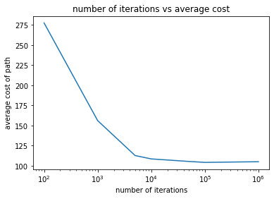
The average path cost decreased linearly as the max allowed number of iterations increased. This was expected. Note the x-axis is plotted on a log-scale and the y-axis is plotted on a linear scale. The path cost was the average path cost over 10 annealing trials except for those with a stopping iteration $n_{iterations}=1e5, 5e5, 1e6$ for which only a single trial was done.

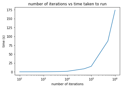
The time taken to run the annealing algorithm increased linearly as the max allowed number of iterations increased. This was expected. Note the x-axis is plotted on a log-scale and the y-axis is plotted on a linear scale. The time taken was the average time over 10 annealing trials except for those with a stopping iteration $n_{iterations}=1e5, 5e5, 1e6$ for which only a single trial was done.

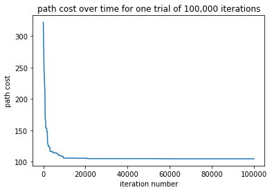
This graph shows the convergence of the annealing algorithm over time for a single trial where the maximum number of iterations was $1e5$. The path cost converges rather quickly and possibly not this many iterations was required.

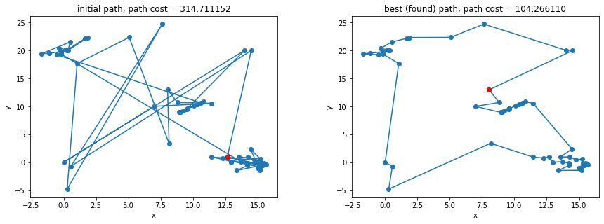
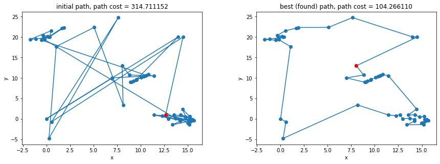
The initial path (arbitrarily in the order given) and the best solution path found are plotted above. While it does not really matter where we start, the start node is colored red just to give a the user a visual start and end point. The final solution had a path cost of $104.266$, a 33% improvement from the initial path shown. While there is no way to know whether this is the guaranteed optimal solution (without searching the entire $n!$ state space), upon visual inspection, the path looks at least close to optimal.

Some drawbacks were that it took a rather long time to converge (100,000 iterations took about 15 seconds, while 10,000 iterations took about 1.5 seconds) and that it took some time and energy to find the constants for the temperature function. There were too many open parameters to tweak and that seemed to be different as the maximum stopping iteration changed. To improve my implementation of the algorithm, I would consider sizing my random changes in random_move based on the size of the temperature $T(t)$. This would make more effective use of the number of iterations, because the size of random change being made would be more likely to make an accepted change. Additionally, I would consider changing and optimizing how I am making random changes. Currently, I am only reversing a random subarray of points (within a solution) and other changes might be more effective and efficient.

Ultimately, the annealing algorithm was very successful and was able to find a good solution within a very reasonable amount of time, but I’d love to continue improving it.