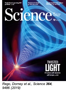
I modified the standard Gerchberg-Saxton (GS) phase-retrieval algorithm to return more information than traditional beam-characterization methods given the same data. Other members of my lab group used the algorithm to analyze their laser beams containing orbital angular momentum (OAM), which resulted in a publication in Science Magazine.

Presentation Paper M^2 Presentation

I worked with David Couch, a graduate student who mentored me for 3 years. This project spun off of a project to create an M^2 beam characterization device and preliminary work was completed at the very end of summer 2019.

Importance

OAM beams are useful in optical communications, imaging, magnetics, quantum information science, and many other fields. For example, light containing OAM was shown to transmit up to 1.6 Tb of information per second-the equivalent of 8 Blu-ray discs per second (Source). Reliable phase detection is essential for the development of future technologies.

Beam-characterization is a necessity for all experiments involving a laser beam and phase contains powerful information that is necessary to completely characterize a laser beam. In order to completely characterize a laser beam (or any light source for that matter), we need both intensity and phase. An intensity profile is relatively easy to obtain; we can simply shine the laser on a camera which will produce a matrix of values. Obtaining phase information is more complicated and involves the use of algorithms.

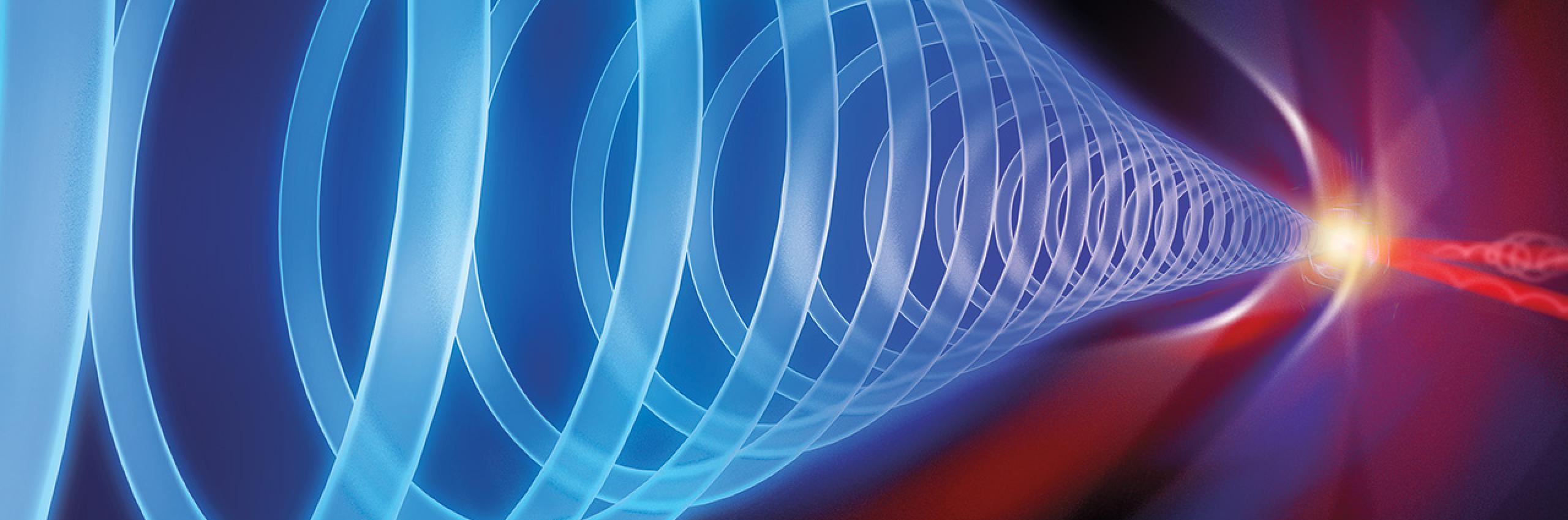
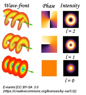
OAM beams

OAM beams are laser beams with a “twisted wavefront”, meaning they contain angular momentum that is dependent on spatial distribution (as opposed to polarization- angular momentum that is dependent on the quantum spin of a photon).

(Source)

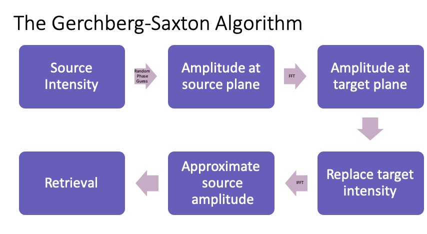
The algorithm

Theory

Having intensity and phase information in one plane allows the propagation of the beam to another plane. In other words, if information about phase and intensity is obtained at one point along the laser beam path, then we also have information about the laser beam at ANY other point. Furthermore, having intensity information in two different planes allows for the calculation of the phase in the two planes.

The original Gerchberg-Saxton algorithm uses an image at the focal point and an image infinitely far away from the focal point to iteratively retrieve the phase of the beam.

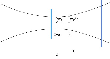
Our algorithm uses an over-sampled intensity measurement. We take 9-30 images with at least half of the sampled points occurring within one Rayleigh range of the focal point (as recommended in the ISO standard for M^2) instead of only two. This oversampling ensures a much more robust and accurate characterization of the beam. There is an optimal solution and additional degrees of freedom that can be used to confirm the result. We also apply a phase perturbation of L = +- 1/2 every 10 iterations for the first 40 iterations, which helps the algorithm to converge more quickly. It also helps to prevent the GS algorithm from getting stuck in local minima.

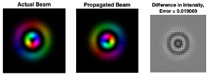
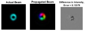
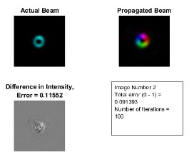
An example retrieval looks like this, with an intensity profile plotted on the left, the retrieved phase overlaid on top of the intensity in the center, and the error on the right.

Handling Wavelength

In original GS and our main algorithm, the retrieval algorithm must know the wavelength of the laser. For a single wavelength, we found the algorithm can reliably determine the wavelength to within about 5 nm.

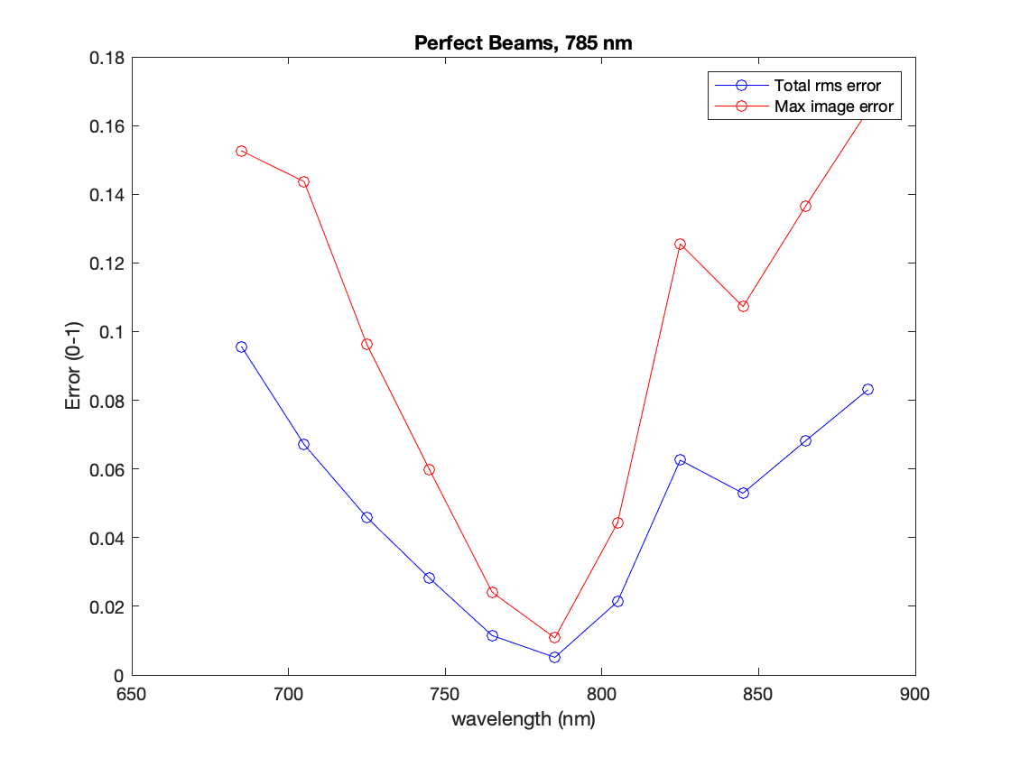
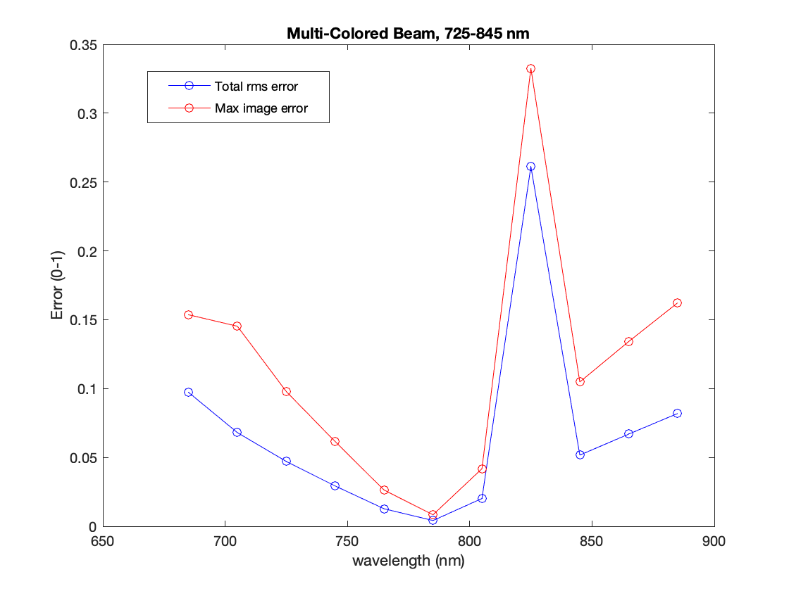
For multiple wavelengths, the algorithm does not perform very well.

Below are example retrievals for when the algorithm is given the incorrect starting wavelength. It clearly converges on incorrect results, but when plotted they turned out to be very beautiful!

Sampling on one side of the focus

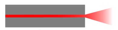
For EUV OAM beams, like the in the Science article, optics have very poor efficiency. Without optics, we cannot get a full profile of the focal point of these beams. Additionally, for many projects it is difficult to access the focal point (say, if it inside a fiber), so it would be beneficial to test if the algorithm works when given only data from planes on one side of the focus. Preliminary tests have shown this looks promising.

Source: ThorLabs

Example Results:

Comparison to Other Techniques

• M^2 uses the same information as the GS algorithm to compute beam divergence characteristics (2 numbers)

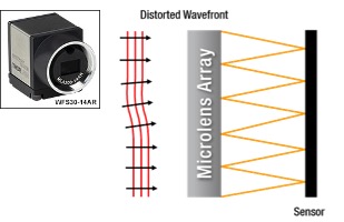
• Shack-Hartmann is an expensive (~$4000) wavefront sensor that can measure OAM content but has low spatial resolution and relatively narrow useful wavelength range (cannot be used in VUV/EUV)

Source: ThorLabs

Conclusion

• We have created a powerful beam characterization device that is capable of comprehensively characterizing a wide variety of beams.
• It is able to gather more information than traditional characterization methods from the same data set and achieve higher resolution
• The algorithm can determine wavelength for a single-wavelength beam
• Preliminary results show difficulty with several wavelengths and with sampling only on one side of the focus

Next Steps

• Analyzing the algorithm performance
• Exploring the capabilities of the algorithm for multi-wavelength handling
• Optimizing for speed and accuracy, and extending this to handling images from only one side of the focus

Code Snippets

GS Algorithm

% MODIFIED 6/9/2019

function [Amps_rtrv, Ints_rtrv, Phase_rtrv] = GSPhaseRetrieval(images, locations, beta, numIterations, wavelength, pixelsize)

%%% Rename Variables

lambda  = wavelength*1e-9;  %convert nm to m
y = pixelsize*1e-6*(1:imssize(1));  %convert um to m
x = pixelsize*1e-6*(1:imssize(2));
z = locations*1e-3; %convert mm to m
images = images./sum(sum(images,1),2); %normalize images

%%% Given I, z, wavelength
amp = sqrt(abs(images));
phase = 0;
beams = complex(zeros(length(y),length(x),length(z)));
beams = amp.* exp(1i*phase); %sets up first guess where phase = 0 at all points 
amp1 = amp(:,:,1);

beam1 = beams(:,:,1);  %initial guess

error = nan(numIterations,1); %preallocate
numPlanes = size(images,3);

for i=1:numIterations
    %%% Give a little OAM content
    if i < 40 && mod(i,10) == 0
        [Y,X] = ndgrid(y,x);
        OAMmat = (X-mean(x)) + 1i*(Y-mean(y));
        OAMmat = OAMmat./abs(OAMmat);
        beams(:,:,1) = beams(:,:,1).*exp((mod(i/10,2)-0.5)*1i*angle(OAMmat)); %add pi/2 OAM content
    end
    rmsError = 0;
    for n=2:numPlanes
        beam = propagate_spw(beams(:,:,n-1), y, x, z(n)-z(n-1), lambda);  %%guess for each image
        diff = amp(:,:,n) - abs(beam);
        rmsError = rmsError + sqrt(mean(abs(diff(:)).^2));
        beams(:,:,n) = (abs(beam)+diff*beta) .* exp(1i*angle(beam)); %replace guessed amplitude with measured amplitude
        %beams(:,:,i+1) = propagate_spw(adjustedBeam, y, x, z(i+1)-z(i), wavelength);
    end
    
    adjustedBeam1 = propagate_spw(beams(:,:,numPlanes), y, x, z(1)-z(numPlanes), lambda);
    diff = amp1 - abs(adjustedBeam1);
    beams(:,:,1) = (abs(adjustedBeam1)+diff*beta) .* exp(1i*angle(adjustedBeam1));
        
    rmsError = rmsError + sqrt(mean(abs(diff(:)).^2));
    error(i) = rmsError;
end

%%% Calculate all beams by propagating first image
I = zeros(length(y), length(x), length(locations));
P = zeros(length(y), length(x), length(locations));
% calcbeams = complex(zeros(size(beams)));
for i = 1:Nimages
    beams(:,:,i) = propagate_spw(beams(:,:,1),y,x,(z(i)-z(1)),lambda);
    error(i) = sum(sum(abs(images(:,:,i)-abs(beams(:,:,i).^2))));
    I(:,:,i) = abs(beams(:,:,i).^2);
    P(:,:,i) = angle(beams(:,:,i));
end

% Save the output.
Amps_rtrv  = beams;
Ints_rtrv  = I;
Phase_rtrv = P;

Simulate beam intensity

The number of pixels Npixels and pixelsize (in m) must be specified.

w0 = 40e-6;    % m, HW1/e2 spot size
x = ((1:Npixels)-mean([1,Npixels]))*pixelsize; %converts to matrix to units of meters and sets the center as 0
y = ((1:Npixels)-mean([1,Npixels]))*pixelsize;
[Y,X] = ndgrid(y,x); %creates 2 matrices, one describing x-distances from 0 and one describing y-distances from 0
RHO = sqrt(Y.^2 + X.^2);
PHI = atan(Y./X) + pi*(X<0) + pi/2;
r = RHO/w0;

E = (sqrt(2)*r).^abs(l)*(1).*exp(-r.^2).*exp(1i*l*PHI); %a matrix describing the field at the focal point

Acknowledgements

This project was funded by STROBE and the NSF and was done as part of the STROBE SURS Program. Thank you to David Couch, Kevin Dorney, Michael Tanksalvala, Matthew Jacobs, Kate Uchida, Dr. William Peters, Prof. Margaret Murnane, Jatinder Sampathkumar, Sadie Stutzman, and Prof. Nicole Labbe.